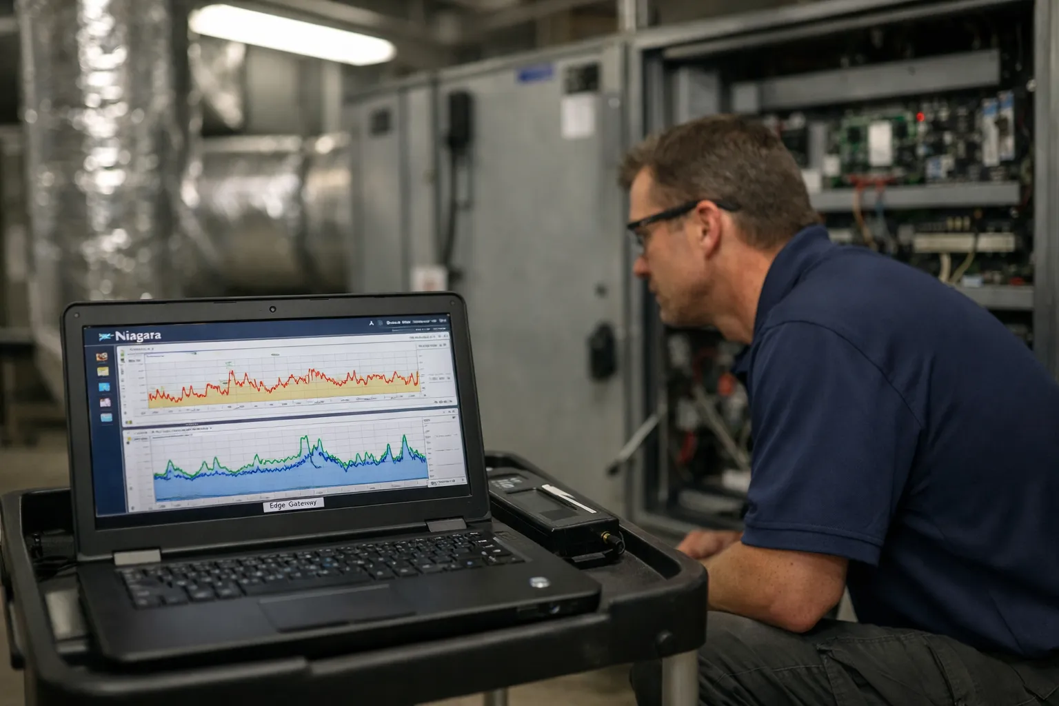
Precision control of HVAC loops remains one of the highest-leverage, low-cost opportunities to improve occupant comfort and reduce energy consumption. This guide walks HVAC enthusiasts and field technicians through a practical, verifiable workflow for tuning PID (proportional–integral–derivative) control loops using building automation system (BAS) trend data and, when appropriate, lightweight machine-learning (ML) tools available in 2026.
Why tune PID loops now?
In 2026 many buildings run legacy PID loops tuned by rule-of-thumb or left at factory defaults. Modern BAS platforms (Niagara, Siemens Desigo, Johnson Controls Metasys, KMC Commander and others) provide high-resolution trends, tighter integration and edge compute that make systematic retuning practical. Correctly tuned loops reduce oscillation, minimize integral windup and shorten settling time — improving comfort and often trimming energy by 3–8% on HVAC equipment through reduced cycling and better staging.
Overview: a practical tuning workflow
- Identify candidate loops and define success metrics
- Collect and clean BAS trend data
- Perform loop characterization (step tests or relay tests)
- Select a tuning method (Ziegler–Nichols, Tyreus–Luyben, model-based, or ML-assisted)
- Implement settings with safeguards and anti-windup
- Validate with acceptance tests and document results
Step 1 — Identify loops and metrics
Not all loops are equal. Prioritize by impact, risk and ease of testing:
- High priority: AHU discharge air temperature, chilled water temperature control, VFD-driven duct static pressure, condenser water pumps, reheat coil control on VAV boxes.
- Medium: Hot-water loop supply temperature, room-level temperature loops with frequent setpoint changes.
- Low: Stable slow-moving loops (e.g., long-run process temperatures) unless misbehaving.
Define success metrics before tuning. Common metrics:
- Rise time and settling time to ±0.5–1.0°F (or ±0.25–0.5°C) for temperature loops
- Overshoot as percentage of setpoint
- Integral of Absolute Error (IAE) or Integral of Time-weighted Absolute Error (ITAE) over a defined period
- Number of control actuator reversals or on/off cycles per hour
Step 2 — Collect and prepare BAS data
Gather 2–7 days of high-resolution trends where possible (1–5 minute resolution). Where you plan active testing, schedule quiet building hours. Export relevant signals:
- Process variable (PV): e.g., discharge air temp, space temp
- Setpoint (SP)
- Controller output (CO): 0–100% command, valve position, VFD speed
- External influences: outdoor air temp, occupancy schedule, valve status, pump run
Clean the data: remove obvious sensor dropouts, apply a median filter for isolated spikes, and align timestamps. For control analysis you want continuous segments where SP is steady or where deliberate step changes will be applied.
Step 3 — Characterize the loop
Two practical characterization approaches:
Passive identification
Use existing disturbances and SP changes in the BAS trend to estimate loop gain and time constants. Tools like Python’s pandas + statsmodels or commercial BAS analysis modules can fit first- or second-order transfer functions. Passive methods are low-risk but can produce noisy estimates if disturbances are weak.
Active step test (recommended)
Apply a controlled step change to the controller output (e.g., increase heating valve command by 10–20% for 10–30 minutes) and record PV response. For VFD or valve actuators respect equipment limits and coordinate with operations. From the step response you can estimate process gain (Kp), time constant (τ), and dead time (θ) — inputs to many tuning rules.
Step 4 — Choose a tuning method
Pick a method appropriate to the loop dynamics and risk tolerance.
- Ziegler–Nichols (classic): Quick but aggressive; tends to produce oscillatory responses good for initial tuning where speed is prioritized.
- Tyreus–Luyben: Slower, more damped than Ziegler–Nichols; better for HVAC where overshoot must be limited.
- Model-based PID (Åström–Hägglund, IMC): Uses fitted first/second-order model and produces less aggressive, robust settings.
- ML-assisted optimization: Use local regression, Bayesian optimization or simple reinforcement strategies to search parameter space safely. In 2026 lightweight tools embedded in edge controllers can recommend gains based on historical data and simulated step responses.
Practical tuning examples
For a first-order-plus-dead-time process (FOPDT), IMC-based PI tuning often yields good HVAC performance:
- Controller bandwidth λ = max(θ, τ/2)
- PI: Kc = (τ / (Kp * (λ + θ))) ; Ti = min(4τ, 8θ)
For a quick on-site approach where you can't identify τ and θ precisely, try Tyreus–Luyben: from the ultimate gain Ku and period Pu (found with relay test or step-up until sustained oscillation), set Kp = 0.312 Ku, Ti = 2.2 Pu, Td ≈ 0.
Step 5 — Implement safely
Implement new tuning parameters with conservative rollout:
- Apply changes to a single loop in a non-critical zone first
- Enable anti-windup and derivative filtering; set CO limits to prevent actuator saturation
- If controller supports supervisory constraints, add rate limits to controller output to protect valves and VFDs
- Log at high resolution for at least 24–72 hours post-change
Communicate with building operations and occupants when testing will occur. Use BAS trends to monitor transient behavior and revert quickly if necessary.
Step 6 — Validate and document
Run your acceptance tests: apply a setpoint step or let the system run through a typical occupancy cycle, then calculate your pre-defined metrics. Example acceptance criteria:
- Settling time reduced by ≥25% versus baseline
- Overshoot ≤1°F for temperature control loops
- Actuator cycling reduced by ≥20% per hour
Document initial and final parameter sets, test conditions (outdoor temp, load conditions), and before/after trend screenshots. Store results in the building’s digital handover file for future tuning cycles.
ML and automation — where it helps and where it doesn’t
By 2026, many BAS vendors provide ML-assisted tuning modules. Use them for:
- Batch analysis across many similar loops — spot underperformers
- Suggesting starting gains based on historical patterns
- Automated A/B testing with safe rollback
Don’t use black-box ML to replace engineering judgment. ML tools are best when constrained (e.g., Bayesian optimization with conservative priors) and combined with simulation-based safety checks.
Common pitfalls and how to avoid them
- Bad sensors: Always verify accuracy and response time of PV sensors before tuning. A noisy or slow sensor ruins tuning.
- Actuator limits and backlash: If a valve or damper is sticky, tuning gains will produce oscillation. Audit mechanical health first.
- Unmodelled cascades: For cascaded loops (e.g., space temp master, valve position slave), tune the inner (fast) loop first, then the outer loop.
- Ignoring occupancy and schedules: Test under representative load and schedule conditions. A loop that looks “excellent” at night may fail under daytime load.
Case study: AHU discharge temp loop tuned with IMC and ML validation
Context: A 2016-era office building with a 30,000 cfm AHU had a discharge air temperature loop with visible oscillation and frequent VFD cycling. Baseline data: 7-day trend at 1-minute resolution. Passive analysis identified τ ≈ 8 minutes and θ ≈ 1.5 minutes; process gain Kp ≈ 0.35 °F/%CO.
Tuning approach: IMC-based PI tuning produced conservative gains: Kc = 0.9, Ti = 12 min. After implementation with anti-windup and a 3%/min CO rate limit, settling time dropped from ~22 minutes to ~9 minutes and overshoot reduced from 4°F to 0.8°F. VFD reversals fell 35%.
ML validation: A constrained Bayesian optimizer tested ±20% around baseline gains during overnight hours on low-occupancy days, confirming the IMC parameters were near-optimal for energy/comfort trade-offs. Documented savings: modelled annual energy reduction of ~4% for AHU fan energy and reheat load.
Tools and resources
- BAS native trend modules (Niagara Risk Management, Siemens Energy Manager)
- Python toolchain: pandas, numpy, scipy, statsmodels for identification; scikit-optimize or GPyOpt for constrained Bayesian tuning
- Edge/Cloud ML services offered by BAS vendors — use vendor sandbox and validate offline first
- Reference texts: Åström & Hägglund, “Advanced PID Control”; HVAC control commissioning guides from ASHRAE
Checklist for a successful tuning engagement
- Back up original controller settings and trends
- Verify sensors and actuators are healthy
- Collect representative BAS data (1–5 min resolution)
- Choose tuning method matched to loop dynamics
- Implement in controlled, staged manner with rate limits and anti-windup
- Validate against pre-defined metrics and document results
- Schedule revisit at 3–6 months to verify seasonal performance
Closing: tuning as ongoing building care
Tuning PID loops is not a one-off task but part of routine building care. With modern BAS visibility and emerging ML tools, enthusiasts and technicians can systematize tuning to improve comfort, reduce wear on actuators and capture real energy savings. Keep the process conservative, data-driven and well documented — that combination yields reliable, repeatable improvements across any building portfolio.