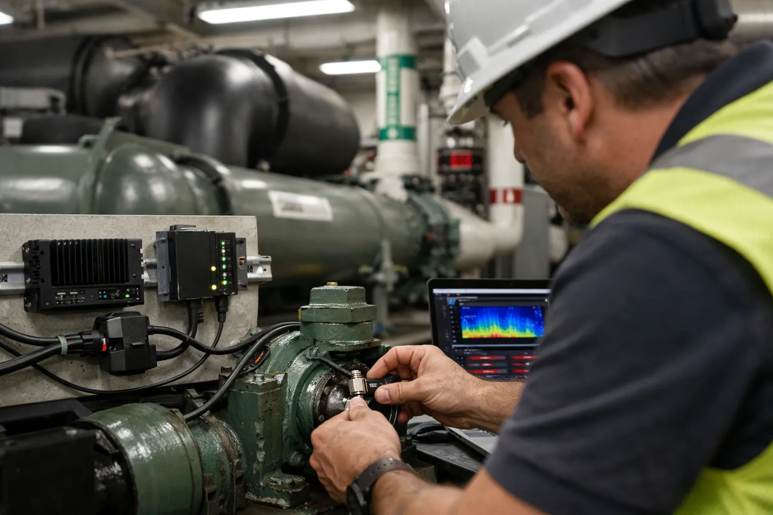
Predictive maintenance (PdM) is now mainstream in industrial sectors; commercial HVAC is next. This guide walks HVAC enthusiasts and field engineers through a concrete, end‑to‑end process to implement an edge‑AI PdM system that detects impending chiller, compressor, motor, and pump faults early — without sending all data to the cloud. Emphasis is practical: what sensors to buy, sample rates, feature engineering, model choices, deployment, integration with BAS/CMMS, validation, and governance.
Why edge AI for HVAC in 2026?
- Bandwidth & latency: Large HVAC sites generate continuous high‑frequency telemetry (vibration, current) — edge inference reduces upstream bandwidth and preserves fast local responses.
- Privacy & reliability: Local inference keeps sensitive operational data on‑premises and continues working through WAN outages.
- Cost: Reduces cloud compute and long‑term data egress costs; common architectures use intermittent cloud training with on‑site inferencing.
- Performance: Modern edge hardware (NVIDIA Jetson Orin NX, Raspberry Pi 5, Intel Movidius/Neural Compute) runs compact models (ONNX/TFLite) with millisecond latency.
Target use cases and expected outcomes
Pick a narrow, high‑value use case for the first pilot. Examples:
- Detect impending screw chiller slide valve sticking and refrigerant charge issues.
- Identify pump bearing wear or misalignment from vibration and current signatures.
- Detect refrigerant compressor unloading failures via harmonic current patterns and discharge temp anomalies.
KPIs to track: mean time between failures (MTBF), unscheduled downtime hours, average detection lead time (days before failure), false positive rate, and maintenance work order reduction.
Step 1 — Define scope, assets, and success metrics
- Inventory assets: e.g., 3 screw chillers (200–300 ton), 8 chilled‑water pumps with VFDs, 40 AHUs with belt drives.
- Choose initial asset class (start with pumps or fan motors — simpler and high ROI).
- Define success: e.g., detect 80% of bearing faults at least 7 days before failure, 10% false positives.
- Stakeholders: facility manager, controls contractor (Niagara/Tridium or Siemens/Desigo), IT/security, and a data engineer or integrator.
Step 2 — Hardware and sensor selection
Match sensors to failure modes.
- Vibration: ICP accelerometers (piezoelectric) for bearings — bandwidth 0.5–5 kHz. For general monitoring, use single‑axis surface accelerometers; for root cause, add triaxial sensors. Typical cost: $150–$450 each.
- Current: Clamp‑on Rogowski or Hall effect sensors for motor current at 2–10 kHz sampling to capture harmonics and transient signatures. Cost: $80–$300.
- Voltage & power: True RMS meters or power meters for harmonic/content analysis (useful for compressor faults).
- Temperature: RTD/TC sensors on bearings, motor windings, refrigerant discharge — 1 Hz sampling is sufficient.
- Environmental: Pressure transducers for refrigerant lines, airflow sensors for AHUs.
- Edge compute: NVIDIA Jetson Orin NX / Xavier, Intel NUC/Edge, Raspberry Pi 5 + Coral TPU for TFLite; choose based on model size and energy budget. Cost: $200–$1,200.
- Data gateway & wiring: Signal conditioners, DIN‑rail ADCs, Modbus/OPC UA/BACnet IP gateways, and surge protection.
Time sync: use SNTP/PTP across devices to align high‑frequency signals to the same timeline.
Step 3 — Data collection & labeling strategy
High‑quality labeled data is the bottleneck.
- Sampling rates: Vibration 4–10 kHz for bearing fault signatures, current 2–10 kHz for transient analysis, temperature 1 Hz.
- Data storage: Edge ring buffer (e.g., 24–72 hours of high‑freq raw) with aggregated summaries (FFT, RMS, crest factor) forwarded to on‑prem historical store (InfluxDB, TimescaleDB) for long‑term trend analysis.
- Labeling: Tie sensor windows to maintenance logs and work orders in CMMS (UpKeep, Fiix, IBM Maximo). For initial supervised models, you need at least dozens of confirmed fault events; where labels are scarce, use anomaly detection.
- Event capture: Implement automatic circular recording triggered by threshold exceedance or scheduled snapshots to preserve pre‑fault windows.
Step 4 — Feature engineering & baseline analytics
Before training models, extract domain features:
- Time‑domain: RMS, peak, kurtosis, skewness, crest factor, envelope RMS.
- Frequency‑domain: FFT band energy (e.g., 1×, 2× shaft speed harmonics), sideband energy for bearing defect frequencies, spectral centroid.
- Current features: THD, individual harmonic amplitudes, transient slope, phase imbalance.
- Cross‑features: vibration-to-current ratios, temperature deltas, power factor shifts.
Use baseline statistical rules (trend thresholds, exponentially weighted moving average) to seed alerting and to provide interpretable fallback rules during ML cold start.
Step 5 — Model selection and training
Pick model families based on label availability:
- Supervised classification/regression (when labeled faults exist): lightweight CNNs on spectrograms, Random Forests on hand‑engineered features, or gradient boosting (XGBoost/LightGBM). Export as ONNX or TFLite.
- Unsupervised anomaly detection (limited labels): autoencoders on feature vectors or time‑series (LSTM/TCN autoencoders), Isolation Forest, or deep SVDD for novelty detection.
- Hybrid: anomaly detector flags potential events; an interpretable classifier refines and scores remaining events.
Training workflow:
- Preprocess: normalize per asset and per sensor type; remove mains hum if needed.
- Cross‑validate on time splits to avoid leakage (train on earlier months, test on later months).
- Use explainability tools (SHAP, feature importances) to ensure models rely on sensible features.
Step 6 — Edge deployment and inference pipeline
- Model export: convert to ONNX or TFLite; quantize (int8) for speed and small footprint.
- Runtime: ONNX Runtime, TensorFlow Lite, or PyTorch Mobile on edge. Use containers (Balena) or system services for robust startup.
- Data flow: sensor ADC -> preprocessor (windowing + FFT) -> model -> local rule engine -> alert aggregator.
- Local actions: immediate local alerts to on‑site technicians, automatic derating via BAS (with safety checks), and push of pre‑fault clips to cloud or central server for review.
- Telemetry: only send events, model confidence, and compressed feature summaries upstream to reduce bandwidth.
Step 7 — Integration with BAS and CMMS
Actionable PdM needs to connect to building controls and maintenance workflows.
- BAS integration: use BACnet/IP or OPC UA for two‑way commands. Implement conservative interlocks: PdM suggestions require human approval unless in automated emergency fallback (e.g., emergency shutdown).
- CMMS integration: auto‑create a work order with asset ID, recommended action, confidence score, and attached sensor snapshots. Use REST APIs (UpKeep/Maximo) or middleware.
- Dashboards: Grafana/Chronograf for trending; include diagnostic plots (spectrogram, current harmonics) in the work order PDF.
Step 8 — Validation, tuning, and operationalizing
Run the system in shadow mode for 60–120 days before autonomous actions.
- Validation: measure precision/recall on real incidents; track detection lead time vs actual failure.
- Human‑in‑the‑loop: have technicians confirm alerts and annotate outcomes to incrementally improve labels.
- Tuning: adjust thresholds, retrain models quarterly or after each confirmed event, and implement a data versioning system (DVC) for reproducibility.
Step 9 — Cybersecurity, privacy, and safety
- Network segregation: place edge devices on an OT VLAN with strict firewall rules. Avoid exposing BAS to the public internet.
- Secure comms: MQTT/OPC UA/TLS with mutual auth, certificate rotation, and VPN for cloud connections.
- Access control: RBAC for dashboards and CMMS. Log all model inferences that trigger actuation.
- Standards: follow NIST SP 800‑53 and IEC 62443 guidance for ICS security.
- Safety: any control actions resulting from PdM must pass mechanical and electrical interlocks and be approved by licensed personnel. Refrigerant work still requires certified technicians (EPA 608 in US).
Step 10 — Business case and ROI estimate
Quick ROI template (example): retrofit a campus with 6 chillers and 30 pumps.
- Costs: sensors & wiring $25k–$60k, edge hardware and gateways $6k–$20k, initial integration & engineering $40k–$100k, yearly support & cloud services $10k–$25k.
- Savings: avoiding two major compressor replacements ($40k–$120k each), reducing unscheduled downtime ($10k–$50k events), and optimizing energy through early coil cleaning — typical first‑year savings often exceed 1.5–3× initial spend on pilot projects.
- Payback: many pilots see payback in 12–24 months when targeted at high‑value rotating equipment.
Practical pitfalls and mitigation
- Pitfall: insufficient labeled failures. Mitigation: use unsupervised models and prioritize assets with historical faults.
- Pitfall: noisy wiring & poor time sync. Mitigation: use shielded cabling, DIN‑rail ADCs close to sensors, and PTP/SNTP.
- Pitfall: unrealistic alerts (alarm fatigue). Mitigation: tune thresholds, require multiple correlated signals to trigger high‑priority alerts, and present confidence scores.
- Pitfall: integration paralysis with BAS vendors. Mitigation: start with read‑only data feeds and CMMS write API before attempting control actions.
Case example: 200‑ton chilled water plant retrofit (concise)
Scenario: mid‑sized office campus with 3 screw chillers, 12 pumps, VFDs, and an existing Niagara BAS.
- Pilot assets: two chilled‑water pumps + one chiller gearbox bearing. Install surface accelerometers on pumps, clamp current sensors on VFD outputs, and RTDs on bearing housings.
- Edge: Jetson Orin NX handling FFTs and a small CNN; preprocessing done in C++ for low latency; MQTT secure bridge to central server.
- Labeling: used last 24 months of CMMS logs to extract 6 confirmed pump bearing failures for supervised fine‑tuning; supplemented with synthetic bearing defect datasets for augmentation.
- Outcome (12 months): detected 5 bearing degradations with average 9 days lead time; avoided two forced shutdowns; pilot costs $38k, estimated avoided repairs and lost productivity $95k.
Next steps for enthusiasts
If you’re an HVAC pro starting this journey:
- Start small: choose one asset type and one building for a 3–6 month pilot.
- Partner with a controls integrator with BAS and IT security experience.
- Collect high‑quality pre‑fault footage now — you’ll thank yourself when a model needs good examples.
- Document every maintenance event and link it to sensor data in your CMMS.
Edge AI PdM for HVAC is now accessible with commercial off‑the‑shelf sensors, affordable edge compute, and mature lightweight ML frameworks. The technical effort is real, but a focused pilot that follows the steps above can rapidly demonstrate value and scale across portfolios. For HVAC enthusiasts, the intersection of vibration diagnostics, power analysis, and on‑site inference offers a rewarding path to longer equipment life, fewer emergency repairs, and a more data‑driven facilities practice.